Lately I’ve been investing a lot in the infrastructure and cloud computing capabilities of my company. Now, we can deploy any containerized application —that includes most open source projects out there—; and, we’re also running out of money. At most our current runway can cover a few more months of our cloud infrastructure, thus we need to start making money somehow.
On the application side of things, we’ve developed a prototype to help video creators and animators. This app is called PixelMux, and currently is capable of generating talking head videos or animating faces in Maya. In its current form it is not yet an MVP, therefore, we cannot sell it.
As a side note, if you want to test our GenAI prototype go to PixelMux, upload a portrait image and short voice clip to animate it.
Given that we cannot commercialize our app prototype yet, we’ve decided to sell our cloud computing capabilities by operating open source projects with a usable license. An example of such tool is Twenty, an amazing CRM for startups, with a GNU license that covers most of its features. The only features not under a GNU license at the time of this writing are “multiple workspaces”, and “billing”.
I don’t want to use our resources (mostly time) to get Twenty to market, because focus is a non negotiable for me. Consequently, we found someone willing to take the risk of selling the CRM in Latam by investing around USD $60.000 into a joint venture. Some details on this initiative are still being negotiated, in particular, the investor wants data on Twenty’s performance in other markets.
Getting sales data of a private company is quite hard (if not impossible), hence we’ve decided to present a proxy to adoption and interest with the goal of helping the investor better understand the potential of the product in Latam. That proxy is data from the community, specifically stargazers of Twenty’s Github repository —people who’ve starred the repo—, and it is my responsibility to create a proper report for the investor.
After some hacking, I managed to get all of the personal (public) information of the stargazers along side the date in which they starred the repository. The only issues with the data, is that the location information of the user does not have standard format, and there is a missingness percentage of around 47%. That being the case, I need to first pre-process the location string to get standard city / country / region values, and then use imputation methods to fill in the blanks.
For the first problem, I decided to batch locations and query an LLM for a standard transformation. Something like, “tell me what’s the country and region of {location}”; one of the main issues with this approach comes from the data’s size. As of now, there are approximately 36.5k stargazers where 19.3k have a location. Just having a few thousands data points is not necessarily problematic, the difficulty comes from the limits of LLMs to process large lists —I must use relatively small batches—; moreover, their APIs have somewhat of a low rate limit, hence, I need something to control the amount of requests per second.
To avoid creating a custom rate limiter HTTP client —I have a few of those implemented in python, but LLMs are not you’re standard API as they have both “request” and “token” limits. Also, I’m very lazy—, I decided to use LiteLLM to handle connection throttling for me.
After a few hours of coding, debugging, and what felt like ages waiting for the LLM to parse all locations, I finally managed to get workable cities and countries strings. At this point, I was ready for some statistical modeling.
A simple solution to the missing data problem was to assume missing and observed sets have the same distribution, then sample from the observed distribution and impute. Nevertheless, I wanted to do some real modeling for fun. For the remainder of the post, I will focus on the statistical model used for imputation.
Mathematical Definitions
As previously mentioned I’m working with stargazers’ data, primarily composed of a starred date and user location. Let’s begin by defining $\tau(s) \in \mathbb{R}$ and $\ell(s) \in L$ as the date and location for a stargazer $s \in S$, respectively. In addition, to make the dates easier to work with, let’s construct a set of non-overlapping time windows defined as
$$ t_i := (T_0 + (i - 1)w, \; T_0 + iw], \qquad i = 1,\dots, N $$
Where $T_0$ is the date in which the repository was created, $T_0 + Nw$ is roughly the latest starred date, and $w$ is a predefined time window —say one month—.
Also, let’s create a few random variables to better represent the data. Given that I’m interested in the geographical and temporal growth of Twenty’s community, let
$$ \begin{align*} X_i(\eta) = \sum_{s \in S} I_{\{ \ell(s) = \eta \}} I_{\{ \tau(s) \in t_i \}}, \newline Y_i = \sum_{\eta \in L} X_i(\eta). \end{align*} $$
Where $\eta \in L$ is a location, e.g., a city or country; and, $I$ is the indicator function.
Now I have this set of random variables that count the number of stargazers across time and geography, and, to impute the missing data, I want to figure out whether $p_i(L) = \frac{X_i(L)}{Y_i} \sim p_j(L) = \frac{X_j(L)}{Y_j}, \ \forall i, j$. That is, answer the question: has stargazers’ geographical distribution remained the same across time?
If the geographical distribution has not significantly changed over time, I can impute the missing data using the basic model previously described; otherwise, I might have to include some auto-regressive or state-space structure.
Observed Data Distribution
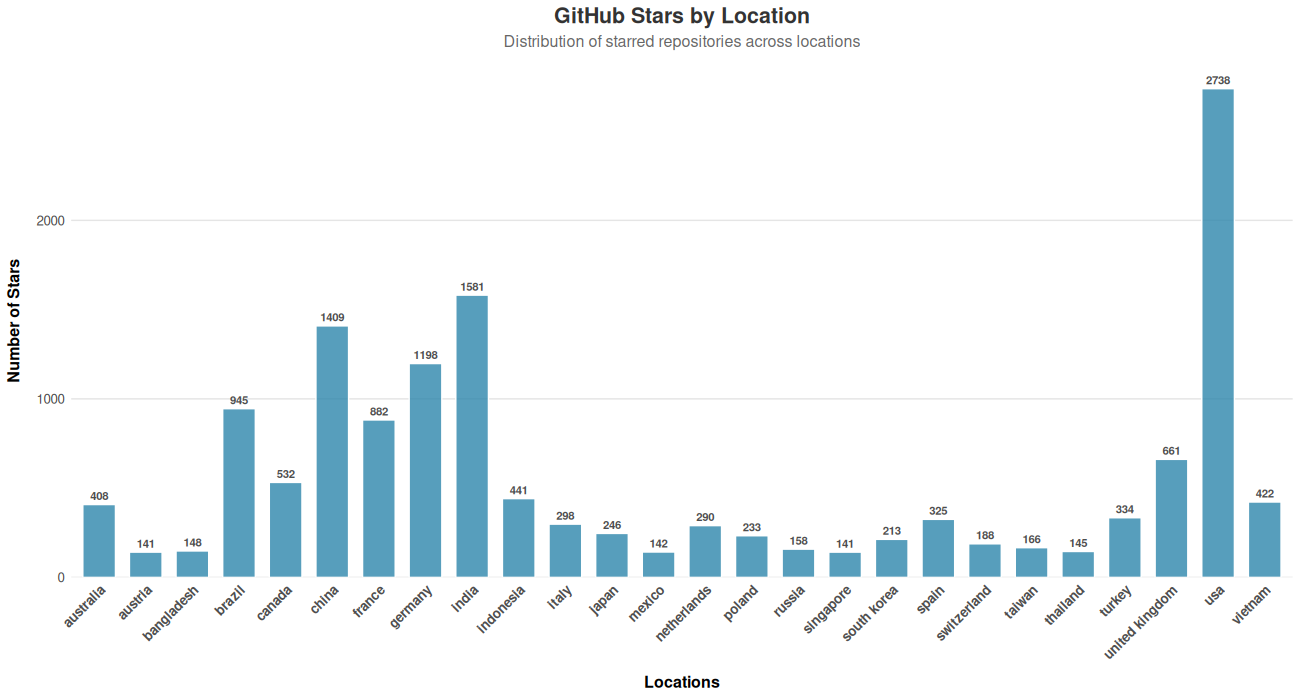
One of the first things I looked into was the overall distribution of stargazers by country. In total there are 163 unique countries, but 80% of the stargazers are located in just 26 countries. To make the figure simpler, I used those 26 countries (Fig. 1).
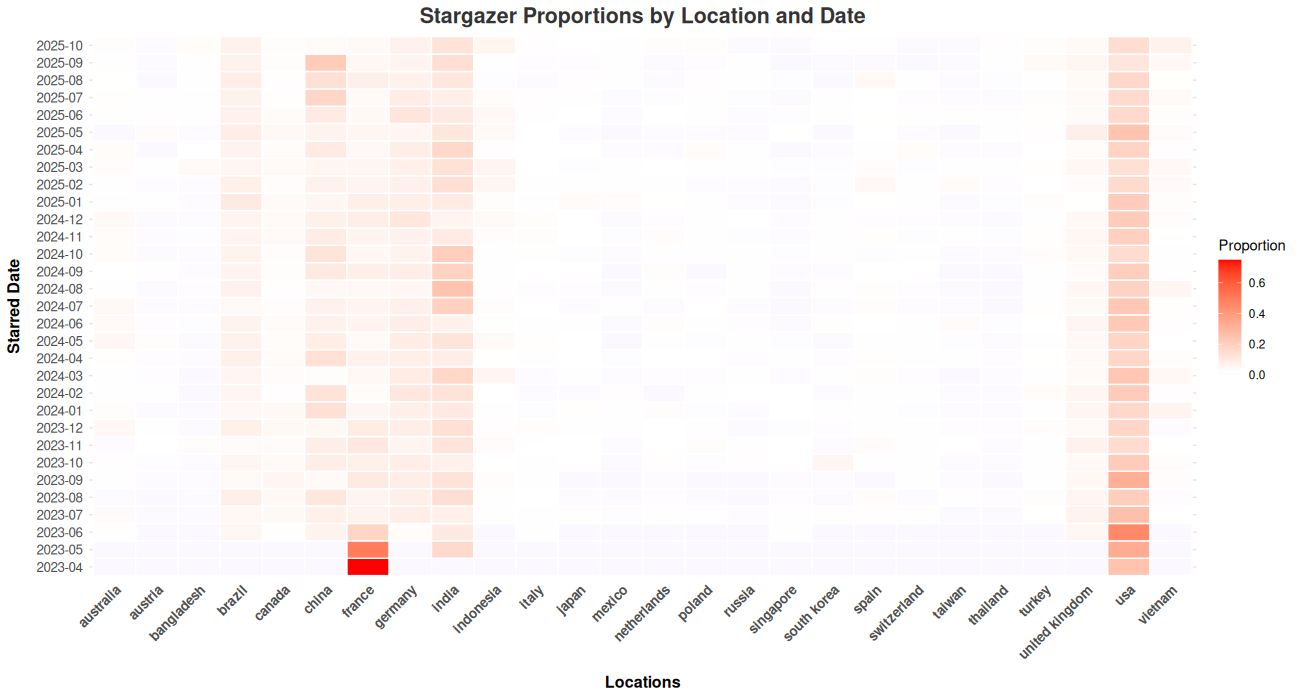
Now, to get some visual queues on stargazers distributions across time, I created a heatmap from a proportions contingency table (Fig .2). This figure shows somewhat homogeneous distribution over time, in markets like the US or France, after removing some of the earliest months of operation. On the other hand, there are a few locations that show an increasing trend in adoption over time, like Brazil, India and China. This suggest the distribution is non-stationary and the use of an auto-regressive or state-space structure is better suited for the data.
Imputation Model
For the imputation model, I decided to use a state-space model, given there exist latent dynamics that evolve over time and affect the observed outcome: stargazers and their geographical location. e.g., Twenty’s go to market strategy is not directly observed in the data, it updates over time based on what’s learned on each time step, and it affects how the project’s community grows.
Mathematically, we can describe stargazers count using the following state-space model:
$$ \begin{align*} X_i(L) \mid f_i \sim \text{Poisson}(\lambda_i), \quad log\lambda_i = \mu + \Lambda f_i, \newline f_i = \Phi f_{i-1} + \varepsilon, \quad \varepsilon \sim N(0, Q), \newline f_1 \sim N(a_1, P_1) \end{align*} $$
Also, let $m := \lvert L \lvert$ be the total number of locations in the observed stargazers data.
Then,
- $f_{i} \in \mathbb{R}^q$, with $q \ll m$, is the latent dynamic factor representing unobserved covariates like Twenty’s go to market strategy,
- $\Lambda \in \mathbb{R}^{m \times q}$, are factor loadings representing the relationship between the latent dynamic factors and log locations count,
- $\mu \in \mathbb{R}^m$, are the log expected count for each location,
- $\Phi \in \mathbb{R}^{q \times q}$, is a transition matrix,
- $\varepsilon \in \mathbb{R}^q$, is some Gaussian noise driving smooth state transitions, and
- $a_1 \in \mathbb{R}^q, P_1 \in \mathbb{R}^{q \times q}$ are assumed to be known constants.
At this point of the story, I had to take a step back as I’d never really worked with this type of models. A simple solution was to use the DynamicFactorMQ class to get a quick output; yet, I was here to have fun and wanted to understand the mathematical structure of the model, so I decided to spend a few hours reading this book. After a while, I figured everything I had to know could be reduced to an efficient way of updating the knowledge of the system as observations arrived (filtering), and estimation (fitting) techniques to get model’s parameters.
Model Fitting
After many more hours, I realized that the model I’m working is a Poisson model, thus regular filtering techniques do not work and am running out of time. For the time being, I will be using the Laplace-EM algorithm, which is an older algorithm that requires computing gradients w.r.t all latent states jointly —inverting large matrices— and can be computationally expensive, yet is simple and my current dataset is small so I can afford the time complexity.
Expectation Maximization
The first step for any Expectation Maximization (EM) algorithm, is to get the functional form of the expected log likelihood function with respect to the posterior; for our specific model, we have
$$\varphi(\theta \mid \hat{\theta}^{(r)}) = E_{f_{1:N} \mid X_{1:N}, \hat{\theta}^{(r)}}[\log p(X_{1:N}(L), f_{1:N} \mid \theta)]$$
where $\theta = (\mu, \Lambda, \Phi, Q)$. For now let’s focus on the data and transition likelihoods.
$$ \begin{align*} p(X_{1:N}(L), f_{1:N} \mid \theta) = p(X_{1:N}(L) \mid f_{1:N}, \theta) p(f_{1:N} \mid \theta) \newline = \prod_{i=1}^N p(X_i(L) \mid f_i, \theta) p(f_1 \mid \theta) \prod_{i=2}^N p(f_i | f_{i-1}, \theta) p(\theta), \newline \log p(X_{1:N}(L), f_{1:N} \mid \theta) = \sum_{i=1}^N \log p(X_i(L) \mid f_i, \theta) + \newline \log p(f_1 \mid \theta) + \sum_{i=2}^N \log p(f_i | f_{i-1}, \theta) + \log p(\theta) \end{align*} $$
Writing out the observation likelihood, we get
$$ p(X_i(\ell) \mid f_i, \theta) = \frac{\lambda_{i, \ell}^{X_i(\ell)} e^{-\lambda_{i, \ell}}}{X_i(\ell)!} $$
Where $\lambda_{i, \ell} = \exp(\mu_{\ell} + \Lambda f_i)$.
For simplicity, I assume that $X_i(\ell) \mid f_i \perp X_i(k) \mid f_i, \text{ for } \ell \ne k$. This assumption is reasonable, since all dependence across locations should be captured by $f_i$. With this in mind, the joint distribution for the observations is
$$ \begin{align*} p(X_i(L) \mid f_i, \theta) = \prod_{\ell \in L}\frac{\lambda_{i, \ell}^{X_i(\ell)} e^{-\lambda_{i, \ell}}}{X_i(\ell)!}, \newline \log p(X_i(L) \mid f_i, \theta) = \sum_{\ell \in L} X_i(\ell)\log\lambda_{i, \ell} -\lambda_{i, \ell} - \log X_i(\ell)! \newline \propto X_i(L)^T(\mu + \Lambda f_i) - I^T \exp(\mu + \Lambda f_i) \end{align*} $$
On the other hand, the state transition distribution is given by
$$ \begin{align*} p(f_1 \mid a_1, P_1) = \frac{\exp(-\frac{1}{2}(f_1 - a_1)^T P_1^{-1} (f_1 - a_1))}{(2\pi)^{\frac{q}{2}} \text{det}(P_1)^{\frac{1}{2}}}, \newline \log p(f_1 \mid a_1, P_1) = -\frac{1}{2} \left[ (f_1 - a_1)^T P^{-1} (f_1 - a_1) + q \log 2\pi + \log \text{det}(P_1) \right], \newline p(f_i | f_{i-1}, \theta) = \frac{\exp(-\frac{1}{2}(f_i - \Phi f_{i - 1})^T Q^{-1} (f_i - \Phi f_{i - 1}))}{(2\pi)^{\frac{q}{2}} \text{det}(Q)^{\frac{1}{2}}}, \newline \log p(f_i | f_{i-1}, \theta) = -\frac{1}{2} \left[ (f_i - \Phi f_{i - 1})^T Q^{-1} (f_i - \Phi f_{i - 1}) + q \log 2\pi + \log \text{det}(Q) \right] \end{align*} $$
With this, I’ve defined the functional form of $p(X_{1:N}(L), f_{1:N} \mid \theta)$. Now to properly use this derivation in the EM algorithm, we need to compute it’s expected value w.r.t the following posterior.
$$ p(f_{1:N} \mid X_{1:N}(L), \theta) \propto p(X_{1:N}(L), f_{1:N} \mid \theta) $$
This posterior is not Gaussian because of the Poisson observations, which breaks the EM algorithm, and is the reason why I couldn’t fit the model using regular filtering techniques. To fix this non-conjugate posterior issue, I use a Gaussian approximation constructed with Laplace’s method,
$$ \begin{align*} p(f_{1:N} \mid X_{1:N}(L), \theta) \approx N(\hat{f}_{1:N}, H^{-1}(\hat{f}_{1:N})), \newline \hat{f}_{1:N} = \arg\max_{\hat{f}_{1:N}} \log p(X_{1:N}(L), f_{1:N} \mid \theta), \newline H(f_{1:N}) = \frac{\partial^2 \log p(X_{1:N}(L), f_{1:N} \mid \theta)}{\partial f_{1:N} \partial f^T_{1:N}} \end{align*} $$
To find $\hat{f}_{1:N}$ I decided to use Newton-Raphson iterations —which is a numerical method to find roots using Taylor expansion (up to the second term)—. As such, I had to find the first and second derivatives of $\log p(X_{1:N}(L), f_{1:N} \mid \theta)$ w.r.t. $f_{1:N}$. Finding these derivatives was a bit cumbersome as getting nice forms for derivatives of linear combinations is (at least for me) time consuming, but when I finally completed this calculation, I had a nice form to compute the posterior of the latent trajectories $f_{1:N}$ and any expectation with respect to them. With this, everything was ready for the Maximization step of the EM algorithm.
Updating $\mu$ and $\Lambda$
To update the observation distribution parameters $\mu, \Lambda$, it is needed to find such parameters that maximize the expected log-likelihood of the observed counts. The following is the expected log-likelihood:
$$ \begin{align*} \mathcal{L}_{obs} = \sum_{i=1}^N E\left[ X_i^T(L)(\mu + \Lambda f_i) - I^T \exp(\mu + \Lambda f_i) \right] \newline = \sum_{i=1}^N X_i^T(L) \Lambda \hat{f}_i - I^T \exp(\mu + \Lambda \hat{f}_i + \frac{1}{2} \text{diag}(\Lambda \hat{V}_{i,i} \Lambda^T)) \end{align*} $$
Where $\hat{V} = H(f_{1:N})^{-1}$ and $\hat{V}_{i,i} = \hat{V}_{[(i-1)q + 1 : iq, (i-1)q + 1 : iq]}$ is the diagonal block matrix.
To maximize it, we take the derivate with respect to $\mu$ and $\Lambda$, where the maximizing values make the log-likelihood equal to zero. For simplicity, the following derivatives are taking with respect to each location individually.
$$ \begin{align*} \frac{\partial \mathcal{L}_{obs}}{\partial \mu_\ell} \big|_{\mu_\ell = \hat{\mu}_\ell} = \sum_{i = 1}^T X_i(\ell) - \sum_{i = 1}^N \exp(\hat{\mu}_\ell + \Lambda_{\ell}^T \hat{f}_i + \frac{1}{2} \Lambda_{\ell}^T \hat{V}_{i,i} \Lambda) = 0 \newline \frac{\partial \mathcal{L}_{obs}}{\partial \Lambda_\ell} \big|_{\Lambda_\ell = \hat{\Lambda}_\ell} = \sum_{i=1}^N X_i(\ell)\hat{f}_i - \exp(\mu_\ell + \hat{\Lambda}_\ell^T \hat{f}_i + \frac{1}{2} \hat{\Lambda}_\ell^T \hat{V}_{i,i} \hat{\Lambda}_\ell) (\hat{f}_i + \hat{V}_{i,i} \hat{\Lambda}_\ell) = 0 \end{align*} $$
To find these MLE parameters, I reused the Newton-Raphson algorithm code used previously in the Laplace normal estimation of the posterior, by alternating between maximizing with respect to $\Lambda_l$ and $\mu_l$.
Updating $\Phi$ and $Q$ (state transition)
When it comes to the state transition update, it is simpler than the observation model update, as it reduces to a multivariate linear regression of the latent states. This is because the derivative of the expected complete-data log-likelihood for the state transitions is linear with respect to $\Phi$ and $Q$ is just a scaling factor. On the other hand, once the updated parameters for $\Phi$ are obtained, they can be used to estimate $Q$ using the regular residual covariance formula from the fitted multivariate linear model.
$$ \begin{align*} \mathcal{L}_{state} = -\frac{1}{2} \sum_{i=1}^N E\left[ (f_i - \Phi f_{i-1})^T Q^{-1}(f_i - \Phi f_{i-1}) + \log \text{det}(Q) \right] \newline = -\frac{1}{2} \sum_{i=1}^N \biggl\{ \operatorname{tr}(Q^{-1} E \left[f_i f_i^T \right]) - \operatorname{tr}(Q^{-1} \Phi E \left[f_{i-1} f_i^T \right]) - \newline \operatorname{tr}(Q^{-1} E \left[f_i f_{i-1}^T \right] \Phi^T) + \operatorname{tr}(Q^{-1} \Phi E \left[f_{i-1} f_{i-1}^T \right] \Phi^T) + \newline \log \text{det}(Q) \biggl\} \end{align*} $$
Going back to our Laplace approximation of the state trajectories $f_{i:N} \sim N(\hat{f}_{i:N}, \hat{V})$, thus $f_i = \hat{f}_i + \delta_i$ where $\delta_i = f_i - \hat{f}_i$. Now, plugging this for the expectations in $\mathcal{L_{state}}$,
$$ \begin{align*} E \left[f_i f_i^T \right] = \hat{f}_i\hat{f}_i^T + \hat{V}_{i,i} \newline E \left[f_i f_{i-1}^T \right] = E \left[f_{i-1} f_i^T \right]^T = \hat{f}_i\hat{f}_{i-1}^T + \hat{V}_{i,i-1} \end{align*} $$
Once again, the MLE makes the derivatives of the expected log-likelihood zero
$$ \begin{align*} \frac{\partial \mathcal{L}_{state}}{\partial \Phi} \big|_{\Phi = \hat{\Phi}} = \sum_{i=1}^N \hat{f}_i\hat{f}_{i-1}^T + \hat{V}_{i,i-1} - \hat{\Phi} \left( \hat{f}_{i-1}\hat{f}_{i-1}^T + \hat{V}_{i-1,i-1} \right) =0 \newline \frac{\partial \mathcal{L}_{state}}{\partial Q} \big|_{Q = \hat{Q}} = \hat{Q}^{-1}S\hat{Q}^{-1} - N\hat{Q}^{-1} =0 \end{align*} $$
Where $S = \sum_{i=1}^N E \left[ (f_i - \Phi f_{i-1}) (f_i - \Phi f_{i-1})^T \right]$
As previously stated, to fit these parameters I just used regular multivariate regression and got the model residual variances.
Final Remarks
Once all of these derivations were completed and the code was implemented, I created the investor report. Now that all is set and done, I feel like just using the python class would of been a better business decision, i.e., get the results fast and move on; nevertheless, it was quite nice to learn in-depth the inner workings of these type of models… At the very least, it was some good practice for my upcoming qualifying exam (I hope).
If you made it this far, don’t forget to subscribe to my newsletter. Also, why did you make this far?